Author: Jarda Snajdr

  • Parkovací domy na Severním předměstí (1981)

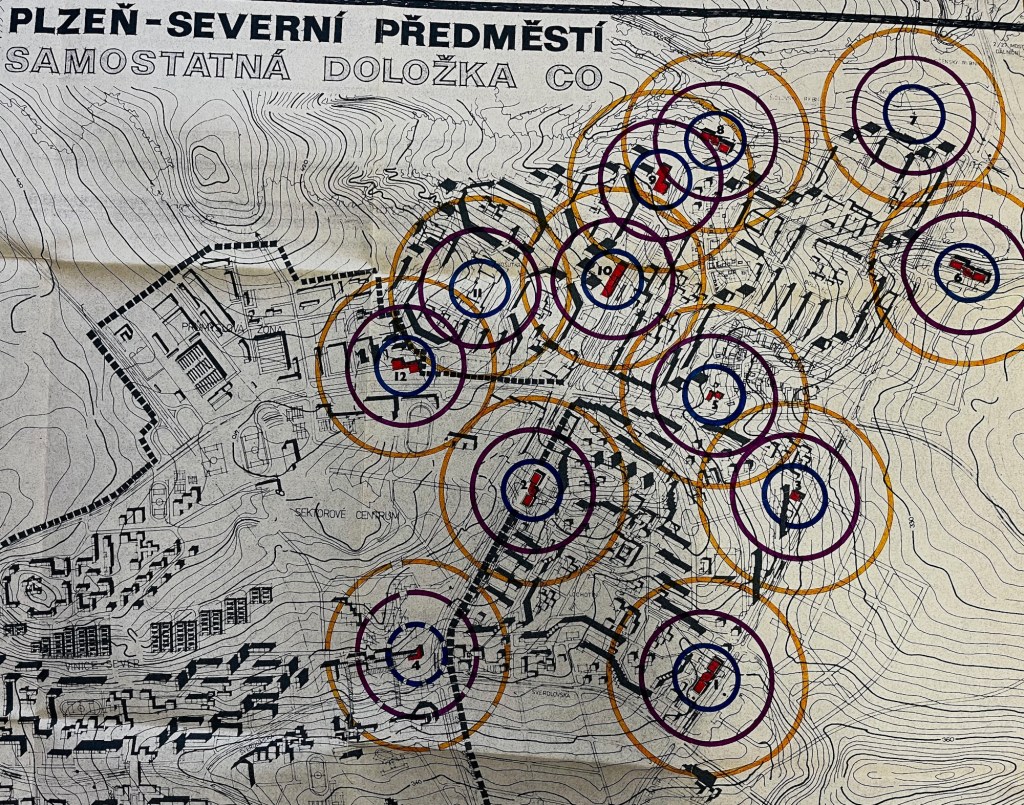
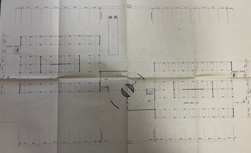
    Parkovací domy na Severním předměstí: nerealizovaný projekt z roku 1981. Na sídlištích Lochotín, Bolevec a Košutka mělo být postaveno cca 10 parkovacích domů, které měly sloužit zároveň jako kryty civilní obrany.

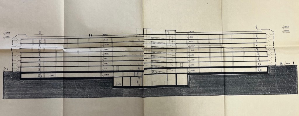
    Pozoruhodná je jejich kapacita: 8 pater, dvě křídla po 60 stáních, celkově pro téměř tisíc aut. Dvakrát větší než např. parkovací dům na Rychtářce. I velikost jednotlivých stání je velkorysá: splňují dnešní standardy, a zatímco do mnohých starších parkovacích domů se dnešní velká auta těžko vejdou, sem by i vaše SUV bez problémů zajelo.

    Toto téma je dodnes aktuální: většina ploch je stále volných, slouží jako normální parkoviště, a platné projekty regenerace sídlišť s parkovacími domy stále počítají.

    Zdroj: Archiv města Plzně, fond Útvaru hlavního architekta

  • Studie dopravy Zbyňka Tichého (1991)

    Studie dopravy z roku 1991, kterou zpracoval arch. Zbyněk Tichý, jeden z hlavních socialistických plánovačů města Plzně od 60. let až do revoluce, a daroval ji městu Plzni (k Vánocům).

    👉 dálnice už je v jižní trase, ve variantách KU (mezi Černicemi a Bručnou) a SU. Skutečná trasa se nakonec ještě hodně změnila a je dnes klikatější: vede dále od Starého Plzence a Radyně, dále od Černic a od Lhoty. Jediné, co odpovídá zcela přesně, je velká křižovatka s přivaděčem od Přeštic.

    👉 silnice 1. třídy vůbec nevedou centrem, ale všechny jsou na okruhu. V mapě označeno jako základní komunikační systém (ZÁKOS) města.

    👉 západní okruh: od Globusu do Radčic stejná trasa jako dnes, ale dále pokračuje blíže městu skrz sídliště Skvrňany a areál Škoda. Široká Lábkova ulice byla již od 60. let plánována jako městský okruh a postavena podle toho, a i průtah Škodovkou pochází ze stejné doby. Obojí je dodnes v územním plánu jako dopravní koridor.

    👉 východní okruh: z Bolevce až do Lobez stejné jako dnes, ale pak vede Sušickou ulicí kolem Božkovského ostrova údolím Úslavy. U Božkovského ostrova si dodnes můžete všimnout širokého koridoru, kam by se čtyřpruh vešel. Dnešní trasa opouští údolí řeky a vede podél železniční tratě.

    👉 jižní část okruhu není v obytné zástavbě Bor (Sukova, 17. listopadu), ale vede opět údolím Radbuzy, kolem Výsluní.

    👉 oba průtahy centrem stále existují, ale už jsou to jen místní komunikace. Zde eufemisticky nazvané “městská sadová třída”. Navzdory mimoúrovňové čtyřlístkové křižovatce uprostřed (Kalikovský mlýn).

    👉 na Lochotíně nová silnice pro auta paralelní s Lidickou ulicí. Těsně pod novou lékařskou fakultou, likvidace židovského hřbitova, kolem Zavadilky (tehdy ještě nezastavěná část), souběžně s elektrickým vedením 110kV.

    👉 počítá se s prodloužením Částkovy a Motýlí ulice, most přes Radbuzu do Doudlevec. To je i v dnešním územním plánu jako “rezerva”.

    👉 velmi zvláštní a agresivní výpadovka I/19 údolím Úslavy a skrz Starý Plzenec, v těsné blízkosti rotundy.

    Zdroj: Státní oblastní archiv v Plzni, písemná pozůstalost Z. Tichého.

  • Lékařská fakulta v Plzni (1945)

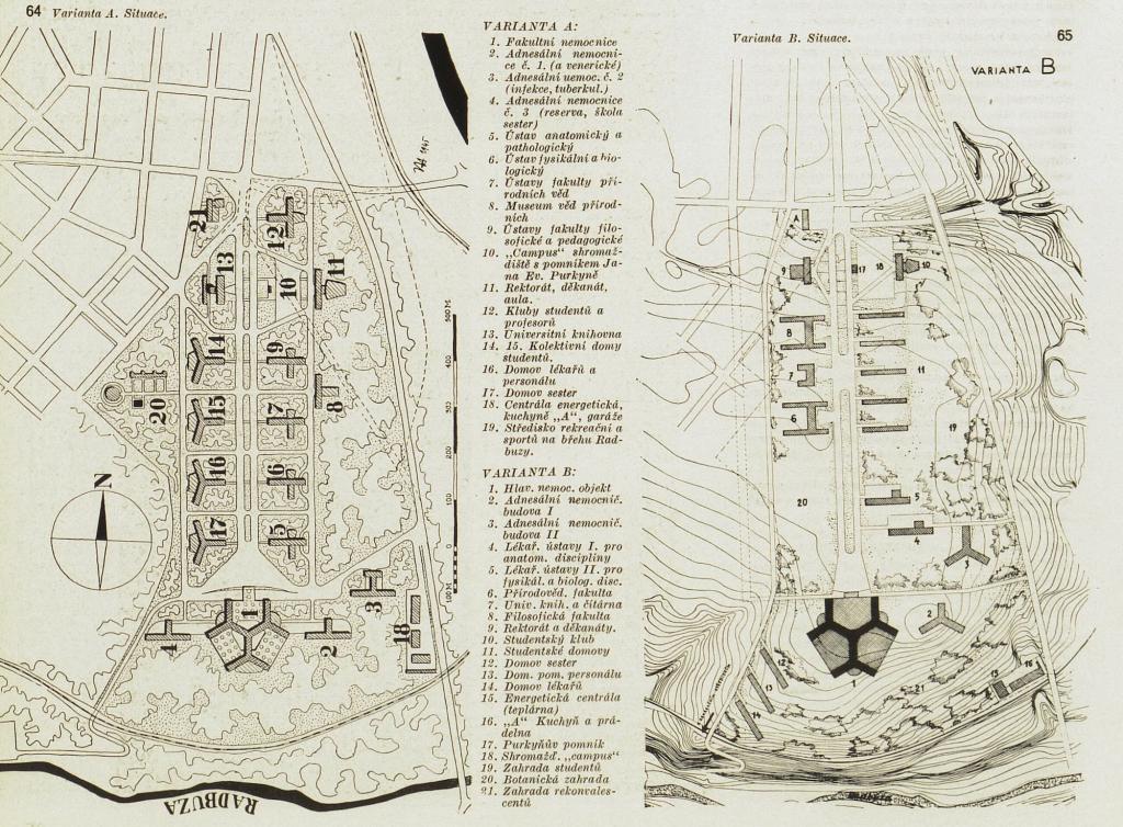
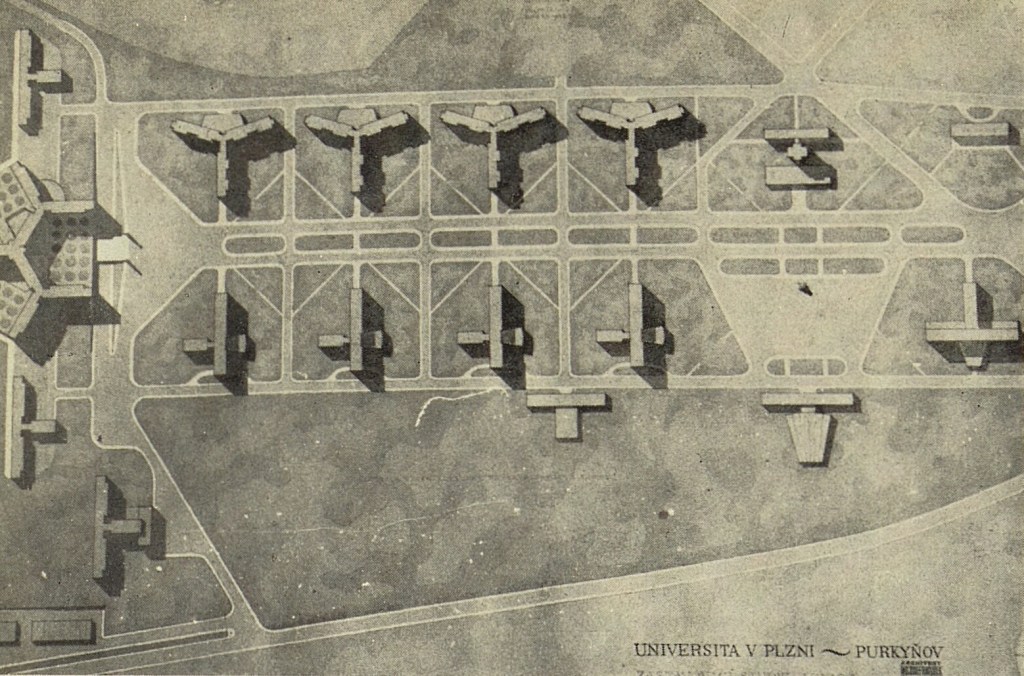
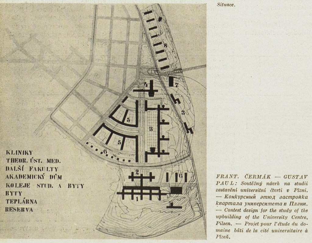
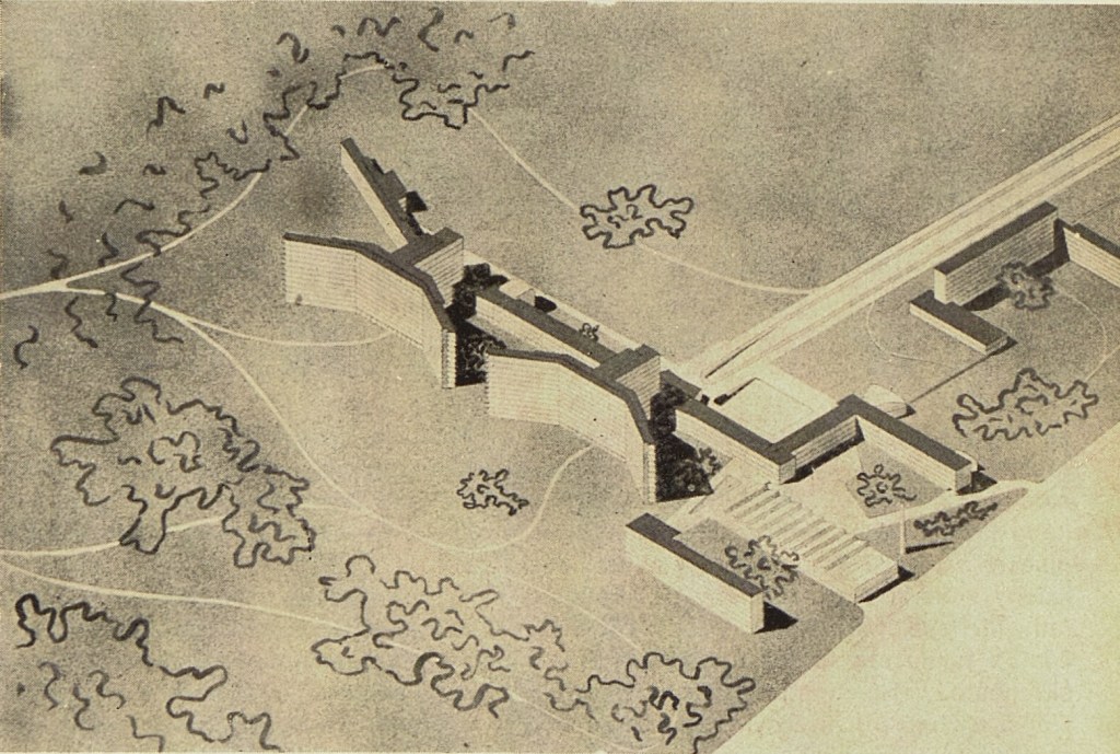
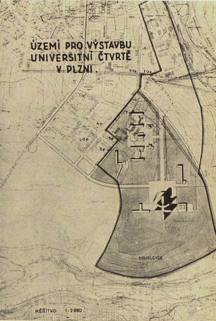
    Lékařská fakulta v Plzni na Borech? V říjnu 1945 byla dekretem prezidenta Beneše zřízena pobočka lékařské fakulty v Plzni a ještě ten samý měsíc proběhla architektonická soutěž na zastavovací studii univerzitní čtvrti na Borech, v místě dnešního sídliště. Čtvrť se měla jmenovat “Purkyňov”.

    V přípravných pracích se už dále nepokračovalo a v roce 1948 vznikl návrh nového územního plánu pro Plzeň, který rozvrhl město téměř přesně tak, jak ho známe dnes, a který umístil lékařskou fakultu a fakultní nemocnici na Lochotín. Ta se začala stavět až po dalších 30 letech a staví se vlastně dodnes.

    Zdroj: Architektura ČSR, ročník 1947. Dostupné v Národní digitální knihovně na ndk.cz.

  • Studie podrobného územního plánu Plzeň severní předměstí (1971)

    Podrobná studie plánu severního předměstí z roku cca 1971, předtím než se začalo cokoliv stavět. V dnešní realitě je mnoho věcí jinak: najdi 100 rozdílů!

    Nepřehlédněte zejména:

    👉 alternativní trasa dálnice D5, nakreslená tečkovaně, údolím Mže blízko centra. Střed Újezda, kostel sv. Jiří, ČOV, pivovarské studny, pod Všemi Svatými, exit u Kalikovského mlýna, …

    👉 dopravní uzel v Lochotínském parku. Dva tunely, paralelní vedení státních silnic, Císařský sál není zbourán.

    👉 velké sídlištní centrum západně od křižovatky Karlovarská/alej Svobody. Zde měly být úřady, poliklinika, knihovna, obchodní dům. Tento projekt zcela zanikl, nepostavilo se z něho nic.

    👉 v nivě Mže je nakreslena spousta sportovišť a občanské vybavenosti. Oddechový park před ZOO, městská hala (na místě dnešního Kauflandu), dostihová dráha, golfové hřiště, přístaviště pro motorové čluny.

    👉 na Mikulce je vyhlídková restaurace “Mikulka”, na svahu dolů k Boleváku opět sportoviště a občanská vybavenost.

    👉 železnice do Prahy je přeložena z Doubravky do oblasti u ČOV a Prioru.

    👉 severní trasa dálnice protíná Senec, nenamáhá se ho objet.

    Originál plánu je 220x140cm velký a je uložen ve Státním oblastním archivu. Digitalizovaný se všemi podrobnostmi a legendou má velikost 20000x12000px.

  • Studie dopravních vztahů v plzeňské aglomeraci (1974)

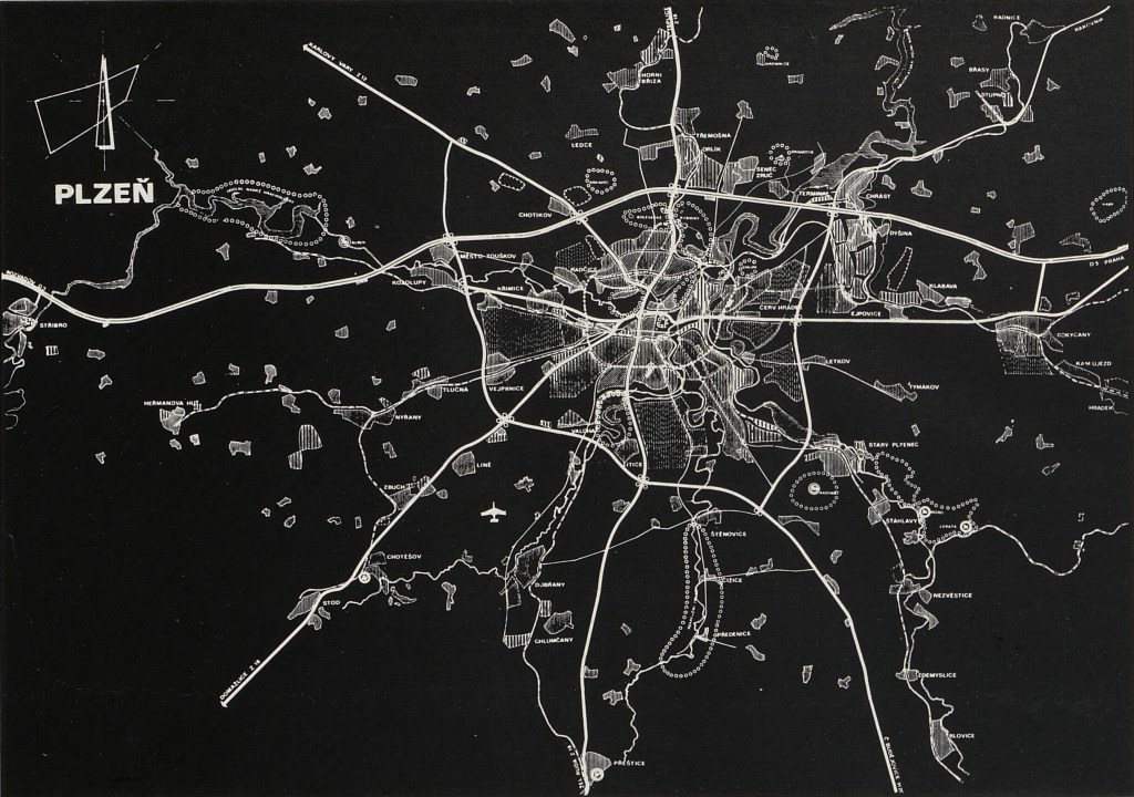
    Studie dopravních vztahů v plzeňské aglomeraci, rok 1974. Za povšimnutí stojí:

    • dálnice D5 v severní variantě: mezi Chrástem a Dýšinou, Druztová, Senec, Orlík, Krkavec, Město Touškov, most přes Mži,další most u Stříbra, kolem něho severně.
    • průtahy silnic 1. třídy přes centrum v plné palbě, superkřižovatka u Kalikovského mlýna.
    • Lidická a Karlovarská nejsou silnice 1. třídy, rozvětvení je širší, přibližně Kotíkovská a Pod Stráží.
    • městský okruh na trase alej Svobody (FN měla být na okruhu) — Nad Feronou — Pecihrádek — Masarykova — Částkova — Motýlí — 17. listopadu — Sukova — Karlov — průtah Škodovkou — Radčice
    • rondel na Roudné nikdy neměl významnější funkci a ani neměl mít, plán na dálnici zde měl jen jepičí život
    • významný vnější (aglomerační) okruh, přibližně na trase silnice 180 a dnešního dálničního obchvatu
    • civilní letiště v Líních

    Zdroj: Miloslav Sýkora, Zbyněk Tichý, Plzeň — založení a stavebně historický vývoj, Architektura ČSR 7/1974. Dostupné v Národní digitální knihovně na ndk.cz.

  • Studie přestavby centrální oblasti města Plzně

    Studie přestavby centrální části Plzně ze 60. let. Kromě historického jádra měla být veškerá ostatní zástavba zbourána (protože je neekonomická, hygienicky závadná a nevyhovující) a nahrazena moderním zářícím zahradním automobilovým městem. Průtah I/5 přímo centrem města, mimoúrovňové superkřižovatky u Kalikovského mlýna a Americká/Klatovská.

    Autorem je architekt František Sammer, žák Le Corbusiera a autor mj. sídliště na Slovanech a Lochotínského amfiteátru.

    Docela velká část byla vlastně realizována: most gen. Pattona, Tyršova ulice, křižovatka u Jána, podchod u nádraží, přemostění nádraží, most Milénia.

    Zdroj: archiv ÚKR a fascinující bakalářská práce Daniely Slepičkové.

  • Chemistry for the Biosciences

    For many years I knew almost nothing about chemistry. I have a fairly good physics background, I know how atoms look like, the nucleus, electrons, orbitals, we even solved the quantum mechanical equations for hydrogen atom in college. But that’s all, I didn’t know anything beyond that. Recently I decided to fix that and read a very nice undergraduate textbook named Chemistry for the Biosciences. Here are my notes. All the visualizations and pictures are done in Wolfram Mathematica.

    Atoms

    The first chapter is about atoms. There is nucleus with protons (positive charge) and neutrons (no charge). Number of protons determines what element the atom is. Hydrogen has one proton, carbon has six, nitrogen has seven, oxygen has eight.

    Every atom has a corresponding number of electrons orbiting around the nucleus. Electrons are negatively charged, are extremely light compared to the nucleus, and the number of protons and electrons is the same so that the atom as a whole has neutral charge.

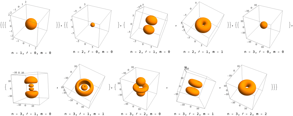
    Electrons are orbiting not like planets, on elliptical trajectories, but in a weird quantum mechanical way. As the number of electrons grows, they are composed around the nucleus in “probability clouds” called orbitals. Here’s how they look like (plotted using the RegionPlot3D function, according to this Mathematica StackExchange answer).

    The bigger and more complex the orbital is, the higher is the energy of the electron. And the asymmetrical orbitals have 3 copies along the x, y, and z axes. If you really want to understand this, they are solutions of the Schrödinger equation for hydrogen atom. The Feynman Lectures on Physics have a chapter on that. It’s volume III chapter 19, at the very end. Not easy.

    Covalent bonds

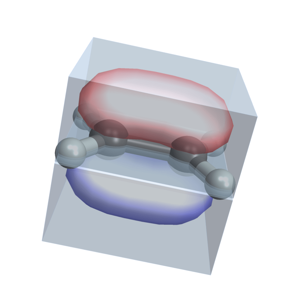
    Most atoms don’t want to be alone. Only the noble gases do. Turns out they are more stable if they share electrons. Each nucleus has no longer its own set of orbital clouds, but some of the clouds merge together. Look at this molecule of ethene (two carbons and four hydrogens) and note how the two carbons share electrons in a common prolonged orbital cloud (I used this Wolfram Demonstration Project, it has examples of several other molecules):

    This sharing of electrons is called a covalent bond and it’s what holds everything together. There is a tremendous amount of details that you can know about covalent bonds. Different elements have different numbers of electrons available for bonding (called valence electrons). That gives the elements different properties and gets them neatly organized into the periodic table. Bonds can be single, double or triple, depending on how many pairs of electrons the atoms share. Different bonds have different strength (energy needed to break them) and length.

    Bonds also determine shape of molecules. In the ethene image above, note how the two electron clouds keep the shape stable: the two “carbon + 2 hydrogens” parts cannot freely rotate, but are locked into one plane. This is extremely important! This is how complex structures like the DNA helix or proteins hold together, without collapsing.

    Non-covalent bonds

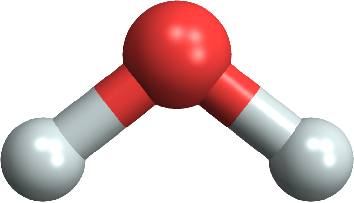
    Look at the water molecule (H2O) and note that it’s asymmetrical:

    MoleculePlot3D["water"]

    What that means is that the centers of the + charge (from protons) and the – charge (from electrons) are not at the same place, but will be slightly apart. That makes the water molecule polar — it’s like a little magnet now. That has many consequences: the molecules tend to hold together, which makes water liquid, and also makes many substances soluble in water.

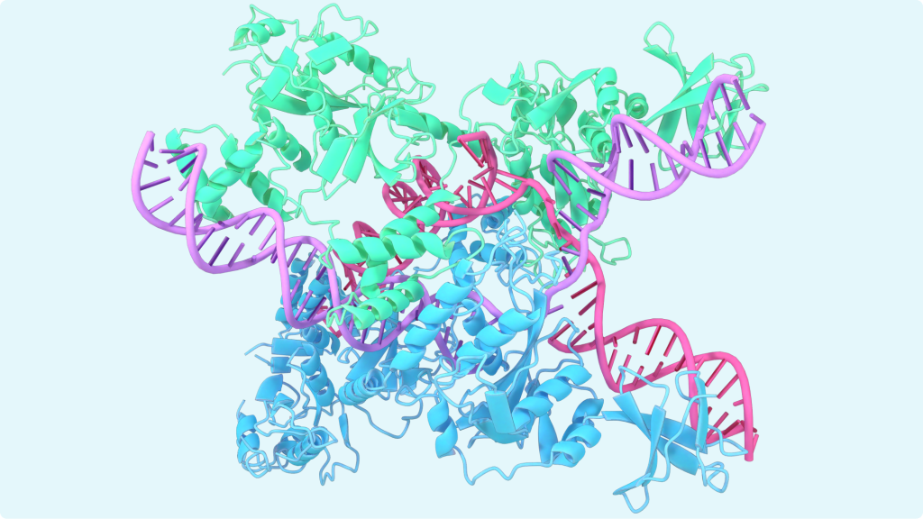
    This weak “magnetic” attraction is called hydrogen bond. It’s order of magnitude weaker than the covalent bond. And you can see it in the double helix structure of DNA!

    Plotted by importing a PDB file from the Protein Data Bank

    The two strands themselves are held together strongly by covalent bonds, but they are connected by a series of weak hydrogen bonds. That means we can separate them easily, and also the hydrogen bonds are very sensitive to the exact location of atoms in the “bases”. Only certain pairs of bases will “click” together. The bases are of four types (ACGT) and only the AT and GC pairs are compatible. That’s the principle for encoding information in DNA.

    This moment is I think one of the pinnacles of the book: you can use the material you learned so far to suddenly understand something very complex and fundamental.

    Building organic molecules

    Now when we are sufficiently familiar with atoms and bonds we are ready to start building larger and larger organic molecules.

    Hydrocarbons

    The simplest ones are hydrocarbons: chains of carbon atoms with attached hydrogens. Here are hydrocarbon molecules with chain lengths from 1 (methane) to 8 (octane):

    MoleculePlot3D /@ {"methane", "ethane", "propane", "butane", "pentane", "hexane", "heptane", "octane"}

    They are so simple that they are useful mainly for burning. Fossil fuels are composed mainly from them. The shorter ones (methane, …) are in gas form, and are known as natural gas. Longer hydrocarbons (up to octane) are liquid and make up gasoline, used to power cars. Even longer hydrocarbons are called kerosene and are used by airplanes and rockets.

    Functional groups

    Hydrocarbons start to be more interesting when we replace the hydrogen atoms with other groups of atoms, called functional groups. Here are four molecules where a hydrogen is replaced with:

    • an -OH group (called hydroxyl) to create an alcohol (methanol)
    • an =O group to create an aldehyde (formaldehyde)
    • an -NH2 group to create an amine (methylamine)
    • a -COOH group to create an organic acid (acetic acid)
    MoleculePlot3D /@ {"methanol", "formaldehyde", "methylamine", "acetic acid"}

    These functional groups react with each other in various ways, and can be combined to produce an infinite variety of organic compounds.

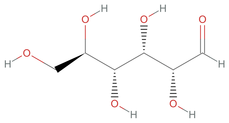
    Consider glucose, which is a six carbon chain with five hydroxyl (-OH) groups and one aldehyde (=O) group:

    MoleculePlot["glucose"]

    Amino acids

    Now let’s have a look at three amino acids, serine, tyrosine and cysteine, and try to decode them. There are parts that they have all in common: it’s the -NH2 (amino) group and the -COOH (carboxyl) group next to it. The remaining parts are called “side chains” and are different. Some of them, like tyrosine, even contain elements like sulfur.

    MoleculePlot[#, highlight]& /@ {"serine", "tyrosine", "cysteine"}

    Theoretically there are infinitely many amino acids, but in nature there are approximately 500 of them, and for human life 22 of them are essential.

    What is interesting about amino acids is that the common parts (the amino and the acid one) can bond together to form so called peptide bond, and can form long chains, called proteins. Depending on which amino acids exactly you bind in what order, a very rich structure emerges, supporting life.

    Proteins

    If you read recent news about AlphaFold, you often see pretty images like this:

    What is that? These are various secondary structures created by long amino acid chains. Sometimes they fold into a helix like structures called α-helixes. You can see them colored in blue and green. You an also see flat zig-zag structures called β-sheets. And nowadays AI is helping us to predict how exactly will the amino acids chains fold and what large-scale 3D structures they will create.

    This is I think the second pinnacle of the book. Putting it all together and understand such a complex structure like a protein.

    Reactions

    Now there are reactions: molecules interact together to form larger molecules, or to divide into smaller ones, replace one part by another.

    After going through various types of reactions, you’ll be able to understand glycolysis: how glucose is broken down in your body and how energy is extracted from it. The energy is stored in molecules called ATP and then transferred in the cell to the place where the energy is released and consumed.

    A very funny part of that is the ATP syntase molecule. It’s a thing that rotates, powered by protons flowing through a small turbine, and the working rotating part is a small robot that grabs an ADP molecule (adenosine di-phosphate), bends it a little, so that an extra phosphate group can easily attach, and produce adenosine tri-phosphate: ATP.

    Chemical analysis

    All the molecules and bonds look very simple, like a magnetic toy for kids, but they are all very small and invisible. We only know about them in a very indirect way. Observing how radiation is reflecting and scattering on them, how they behave in electric or magnetic field, how fast they travel in various mediums. The last chapter describes in detail various analytical methods. And it will make you want to buy a $50,000 HPLC (high-performance liquid chromatography) machine from Agilent.

  • Prefer Jest real timers when testing with React Testing Library

    When testing React components with Testing Library, we should always be using real timers. Fake timers should be a rare exception. Let me offer some reasons why.

    The philosophy of Testing Library is that it runs your React code in an environment as close as possible to the browser. React components are rendered using the default DOM renderer, and a real DOM tree is constructed. The DOM is jsdom, you get very limited CSS styles, no layout or painting, and element dimensions are always 0, but other than that, it’s a pretty good DOM. You perform your test assertions on this DOM, not on some artificial data structure like a component tree produced by react-test-renderer (which is not used by Testing Library at all, except in the react-native flavor). Events are dispatched to this DOM tree, too, TL’s fireEvent is a very thin wrapper around element.dispatchEvent().

    userEvent also tries to be as realistic as possible. Part of that is doing a delay: 0 between events, because that’s close to what the browser also does. Consider this code:

    function handleEvent(e) {
      console.log('one', e.type);
      Promise.resolve().then(()=>console.log('two', e.type));
    }
    return <div onMouseDown={handleEvent} onClick={handleEvent}/>
    

    It logs the mousedown and click events, once synchronously and once after a microtask tick.

    In a browser you get this sequence logged to console:

    one mousedown
    two mousedown
    one click
    two click
    

    Both events are dispatched in separate event loop ticks, and all microtasks scheduled by mousedown run before click is dispatched.

    If you used userEvent.click() with delay: null, you would get a different order:

    one mousedown
    one click
    two mousedown
    two click
    

    Here both mouse event’s are dispatched synchronously, with no tick between them. The microtasks have a chance to run only after both dispatches. That’s why the default delay is delay: 0. It leads to a setTimeout(0) wait between the events, and that leaves room for the scheduled microtasks to finish. The result is more realistic scheduling.

    Generally, Testing Library offers an environment where there’s as little mocking ans as little magic as possible. But Jest fake timers? They are very magical. For example, one striking feature of a test like this:

    function callAfterSecondAndThenAgain(cb) {
      setTimeout(() => {
        cb();
        setTimeout(() => {
          cb();
        }, 1000 );
      }, 1000 );
    }
    
    it('calls the callbacks', () => {
      const cb = jest.fn();
      callAfterSecondAndThenAgain(cb);
      jest.advanceTimersByTime(2000);
      expect(cb).toHaveBeenCalledTimes(2);
    });
    

    is that although the tested function is clearly async, the test is completely synchronous. It’s completely executed within one event loop tick. There is no done callback to be called, no promise returned and awaited. Fake timers keep track of scheduled timeouts and advanceTimersByTime() will synchronously execute them one by one before returning.

    But that’s no longer true when your code uses promises. Promises are always async, they are not affected by fake timers at all. If your async code uses both setTimeout (or setInterval or setImmediate) and promises, fake timers convert it into something that’s half-sync/half-async, and the execution environment is no longer realistic.

    There’s this example code posted on one StackOverflow question:

    jest.useFakeTimers() 
    
    it('simpleTimer', async () => {
      async function simpleTimer(callback) {
        await callback() // without await here, test works as expected.
        setTimeout(() => {
          simpleTimer(callback)
        }, 1000)
      }
    
      const callback = jest.fn()
      await simpleTimer(callback)
      jest.advanceTimersByTime(8000)
      expect(callback).toHaveBeenCalledTimes(9)
    }
    

    With await callback() on line 5, the test fails, calling callback only two times. Removing the await “fixes” it, calling callback nine times. Let’s dissect what happens:

    The await case:

    1. simpleTimer is called, callback is called (call 1)
    2. in next microtask tick (after await), timeout is scheduled. simpleTimer returns.
    3. advanceTimersByTime is called. It sees one scheduled timeout, so it executes it. The timeout callback calls simpleTimer again.
    4. This simpleTimer calls callback immediately and sychronously (call 2), and then immediately returns a promise. That’s because it’s an async function. They execute synchronously until the first await and then return a promise to wait for the rest. The setTimeout call is scheduled for the next microtask tick, after await.
    5. The timeout callback returns (the promise returned by simpleTimer is ignored) and advanceTimersByTime takes control again. There are no more timers schedules, so it returns.
    6. expect check the number of calls to callback and finds two.
    7. The test finishes, and only after it finished, the microtask with setTimeout is executed. A new timer is added to the fake timers queue, but nobody cares anymore: advanceTimersByTime has finished already. The scheduled timer will be probably removed in some afterEach fake timer’s cleanup.

    The no-await case:

    The crucial difference is in step 4. The setTimeout call in simpleTimer will schedule another timer before simpleTimer returns. When control returns to advanceTimersByTime, the timer is already scheduled and advanceTimersByTime sees it. So it will advance timers by another 1000ms and execute the timer callback. This (infinite) loop will continue until advanceTimersByTime spends its entire budget of 8000ms and then it returns. Now callback has been called 9 times.

    That’s fairly complex, isn’t it? You need to track the tasks very carefully to understand this. In a real-life complex code, I’d argue that fake timers with promises become intractable. In the Testing Library codebase, in the waitFor implemenation, the part that handles the fake timers + promises combo, even the library author admits he doesn’t really know what he’s doing:

    It’s really important that checkCallback is run *before* we flush in-flight promises. To be honest, I’m not sure why, and I can’t quite think of a way to reproduce the problem in a test, but I spent an entire day banging my head against a wall on this.

    Kent C. Dodds
  • What’s the point of generators and controls in @wordpress/data?

    At the end of the Motivation for Thunks post we arrived at a thunk function that fetches stuff from a REST endpoint and stores it into state by dispatching an action:

    function fetchFeatures() {
      return async ( { dispatch } ) => {
        const { features } = await window.fetch( '/features' );
        dispatch.receiveFeatures( features );
        return features.length;
      };
    }
    

    This is a good JavaScript function that’s going to do the fetching and receiving, and the return value from the thunk is available as the return value from the dispatch call (asynchronously):

    const count = await dispatch( 'features' ).fetchFeatures();
    console.log( `fetched ${ count } features` );
    

    It all works perfectly. But! For a functional programmer, the fetchFeatures function has a very serious issue: it’s not a pure function. Instead of just returning a value and nothing else, it does side-effects like calling window.fetch or dispatch.receiveFeatures. In a purely functional language like Haskell or Elm, you couldn’t do this at all. So, what if we wanted to write our fetchFeatures JavaScript function in a purely functional way? That looks quite impossible doesn’t it? We want fetchFeatures to be a pure function that merely returns a value, and at the same time we want it to perform network fetches and store updates. You can’t get both at the same time.

    The functional solution, used by Haskell or Elm, and one we’re going to implement now in JavaScript, is to divide the problem into two parts:

    • pure function fetchFeatures that returns descriptions of effects it wants to perform.
    • an effect runtime that reads these descriptions and performs them.

    Now please look carefully at this weird fetchFeatures function:

    function fetchFeatures() {
      return {
        type: 'fetch',
        params: { path: '/features' },
        next: ( { features } ) => {
          return {
            type: 'dispatch',
            params: { action: receive( features ) },
            next: () => {
              return {
                type: 'return',
                params: { value: features.length }
              };
            }
          }
        }
      }
    }
    

    What does it do? It returns an object with shape { type, params, next }. The type of this object could be called Effect and it contains a description of what to do, and what to do next. We want to perform a fetch effect and when it’s done, to call the next callback with the result.

    The next callback again returns the same Effect type, this time requesting a dispatch effect. And so on. Finally the return effect requests to “exit” the program, and to return a certain value to the caller.

    This fetchFeatures function is indeed a pure function. It does nothing but return a value of type Effect. You could write this function in Haskell, too, and actually Haskell programmers really do it this way — only instead of Effect, Haskell names the effect type as IO.

    Now to actually execute the effects, you need an effect runtime that takes an Effect as a parameter and executes it:

    function runEffect( effect, next ) {
      switch ( effect.type ) {
        case 'fetch':
          window.fetch( effect.params.path ).then( body => effect.next( body ) );
          break;
        case 'dispatch':
          registry.dispatch( 'foos' )( effect.params.action );
          effect.next();
          break;
        case 'return':
          next( effect.params.value );
          break;
        default:
          throw `unknown effect: ${ effect.type }`;
      }
    }
    

    This little runEffect function will bring life to our inert and purely functional fetchFeatures function. Running them together like this:

    runEffect( fetchFeatures(), ( count ) => {
      console.log( 'number of features:', count );
    } );
    

    will actually do all the fetching and storing and will print the count of received features.

    This is exactly how Haskell or Elm works, too. The runEffect runtime is hidden from you, because it’s part of the language runtime (or the Elm “kernel”) and is likely written in C. You, as a functional programmer, write purely functional programs that return instances of the IO type (i.e., effects), and the language runtime then looks at what kind of IO did you return, executes it, and calls a next callback, which is encapsulated in a monad type (something like a Promise with a then handler).

    A Haskell example if you’re curious

    Here is an example of a Haskell program that prints a prompt, then reads a line, and then prints a greeting using the line that was just read:

    main = putStrLn "your name?" >>= (
      \_ -> getLine >>= (
        \s -> putStrLn ("Hello " ++ s)
      )
    )
    

    The >>= operator (called bind) is something like a .then method on a promise, or the next callback in our fetchFeatures example. The (\_ -> ...) syntax is a lambda function. This program constructs a structure of IO operations, with callbacks saying what to do next, and returns it from the main program. The language runtime is then responsible for executing these IO operations and calling the callbacks with their results.

    You can try this program out in an online Haskell REPL.

    Doing it with generators

    One ugly thing about our purely functional fetchFeatures function is that it contains a lot of callbacks which are nested and it’s common knowledge that as your program gets more complex these nested callbacks become a hell.

    So, with a little bit of syntactic magic we can convert these nested callbacks into generators. This is a generator version of the fetchFeatures function:

    function* fetchFeatures() {
      const { features } = yield {
        type: 'fetch',
        params: { path: '/features' },
      };
      yield {
        type: 'dispatch',
        params: { action: receive( features ) },
      };
      return features.length;
    }
    

    We are still working with Effect objects, but this time we’re yielding them from a generator. The next callbacks are gone. We are still purely functional, just with a bit of syntactic sugar on top.

    The effect runtime that works with a generator/iterator is a bit more complex, you need to understand generators and iterators in some detail to get it, there is tail recursion etc, and looks like this:

    function doEffect( effect, next ) {
      switch ( effect.type ) {
        case 'fetch':
          window.fetch( effect.params.path ).then( body => next( body ) );
          break;
        case 'dispatch':
          registry.dispatch( 'foos' )( effect.params.action );
          next();
          break;
        default:
          throw `unknown effect: ${ effect.type }`;
      }
    }
    
    function runEffect( effectIterator, next ) {
      function nextEffect( value ) {
        const nextItem = effectIterator.next( value );
        // process return statement
        if ( nextItem.done ) {
          next( nextItem.value );
          return;
        }
        // process effects
        doEffect( nextItem.value, nextEffect );
      }
      nextEffect();
    }


    The code that connects the generator function and the runtime and brings them to life is exactly the same as for the first callback version!

    runEffect( fetchFeatures(), ( count ) => {
      console.log( 'number of features:', count );
    } );
    

    Calling the fetchFeatures() generator returns an iterator (sequence of Effects) and the runtime loops through the iterator and executes the effects.

    If you’re still interested in analogies with Haskell, this generator syntactic sugar we just described is equivalent to the Haskell do notation. Our example program that reads and prints lines would be rewritten to:

    main = do
      putStrLn "your name?"
      s <- getLine
      putStrLn ("Hello " ++ s)
    

    Instead of a series of nested callbacks with the >>= operator, we can write the same program using a do syntax that has a structure similar to async/await.

    The connection to @wordpress/data

    Looking at the fetchFeatures generator, it probably looks familiar to what you’ve seen in @wordpress/data stores and you’re starting to see the connection.

    These generators are pure functions that yield effect descriptions.

    The various effect types that the runtime can handle in the big switch statement are controls and they can be registered dynamically in the @wordpress/data store runtime. There are controls for selecting (reading) and dispatching (writing) to a store, the apiFetch control etc.

    What’s the point of this additional complexity? Well that’s a good question. If you want to write purely functional code without explicit side-effects, then the runEffect or rungen runtime gives you tools to do exactly that and that fact alone is probably a sufficient justification for you.

    If you’re more pragmatic and believe that even code with explicit side-effects can be good code, the answers are not that clear. Some claim that the purely functional code is easier to test and mock. Instead of mocking window.fetch and other random APIs, you create one super-mock for the runEffect runtime and then test your actions against that. There is a well-known Effects as Data talk by Richard Feldman from the Elm team that explains the case for the functional approach in great detail. But I’m personally not very convinced.

    Thunks or Generators?

    A final note about relationship between thunks and generators. These are two concepts that are not on the same level of abstraction I would say. It’s more precise to say that generators are a layer on top of thunks. What I mean by that is that I can write a thunk that is implemented as a generator and effect runtime:

    function* fetchFeatures() {
      const { features } = yield { type: 'fetch', /* ... */ };
      /* ... */
    }
    
    function fetchFeaturesThunk() {
      return ( runEffect ) => {
        return runEffect( fetchFeatures() );
      };
    }
    

    In other words, runEffect( fetchFeatures() ) is a normal, impure and side-effect-ful function call that can be used anywhere in imperative JavaScript code. The runEffect runtime call is the boundary between the purely functional and imperative world.

  • Motivation for thunks

    The redux-thunk package is by far the most widely used middleware in Redux, and now our own @wordpress/data package also supports its own flavor of thunks. Yet the concept of thunks is often poorly understood, the motivation for them is unclear, and they are thought of as something magical.

    In this section I will show how even in a very simple Redux store, without any middlewares, we can run into serious limitations when trying to implement seemingly trivial operations. And how these limitations can be overcome with thunks. We won’t need any asynchronous operations or side effects (i.e., code reaching outside the store) to run into these issues.

    So, look at this @wordpress/data store that has a reducer composed from two sub-reducers with combineReducers, one selector and two actions:

    function defaults( state = {}, action ) {
      if ( action.type === 'SET_DEFAULT' ) {
        return { ...state, [ action.feature ]: action.value };
      } else {
        return state;
      }
    }
    
    function flags( state = {}, action ) {
      if ( action.type === 'SET_FEATURE' ) {
        return { ...state, [ action.feature ]: action.value };
      } else
        return state;
      }
    }
    
    const isFeatureActive = ( state, feature ) => (
      state.flags[ feature ] ??
      state.defaults[ feature ] ??
      false
    );
    
    function setDefault( feature, value ) {
      return { type: 'SET_DEFAULT', feature, value };
    }
    
    function setFeature( feature, value ) {
      return { type: 'SET_FEATURE', feature, value };
    }
    
    register( createReduxStore( 'features', {
      reducer: combineReducers( { flags, defaults } ),
      selectors: { isFeatureActive },
      actions: { setDefault, setFeature }
    } ) );
    

    This store acts as a key-value map for feature flags. I can set a flag value:

    dispatch( 'features' ).setFeature( 'gallery', true );
    

    and then read the flag value with the selector:

    select( 'features' ).isFeatureActive( 'gallery' );
    

    If a feature was not explicitly set with setFeature, it defaults either to false or to a default I previously set with setDefault:

    dispatch( 'features' ).setDefault( 'likes', true );
    

    Now, isFeatureActive( 'likes' ) will return true if I never set it before with setFeature.

    I could also easily implement a resetFeature action that resets a feature flag value back to the default, by adding a new branch to the flags reducer that removes a key from the state map, forcing the selector back to using a default.

    So far, this looks like a textbook example of a Redux store, doesn’t it? A reducer nicely composed from two sub-reducers, a selector that looks at two places in the state tree, several actions with some reducers reacting to them and some ignoring them.

    Our task now will be to add a new action to the store, one that allows us to toggle a feature flag value, i.e., change it to false if it was true and vice versa:

    dispatch( 'features' ).toggleFeature( 'gallery' );
    

    You might be tempted to add a new case statement to the flags reducer:

    if ( action.type === 'TOGGLE_FEATURE' ) {
      return {
        ...state,
        [ action.feature ]: ! state[ action.feature ],
      };
    }
    

    But this is not going to work correctly because the reducer doesn’t know what the old value of the flag really is. When the state (which is state.flags in the combined reducer) doesn’t have a record for the feature flag, we need to look at state.defaults but the flags reducer doesn’t have access to that. It’s not possible to make the following test pass:

    dispatch( 'features' ).setDefault( 'likes', true );
    dispatch( 'features' ).toggleFeature( 'likes' );
    expect( select( 'features' ).isFeatureActive( 'likes' ).toBeFalse();
    

    Wow! The fact that our reducer is nicely decomposed into sub-reducers makes it impossible to implement something as trivial as toggleFeature! That’s quite a serious limitation.

    On the other hand, it’s quite straightforward to implement toggleFeature as a little helper function:

    function toggleFeature( feature ) {
      const active = select( 'features' ).isFeatureActive( feature );
      dispatch( 'features' ).setFeature( feature, ! active );
    }
    

    See, the isActiveSelector can look at both state.flags and state.defaults and we can implement the desired behavior in just two lines of JavaScript code.

    But we can’t package toggleFeature as yet another action on the store, on par with setFeature or resetFeature, because toggleFeature can’t be implemented as an action object processed by a reducer. And that’s a bit silly.

    Here, thunks come to the rescue. What thunks do is that they expand the meaning of what is a Redux action. In addition to treating plain objects with a type field as actions:

    function toggleFeature( feature ) {
      return { type: 'TOGGLE_FEATURE', feature };
    }
    

    a store with thunk support treats functions as actions, too!

    function toggleFeature( feature ) {
      return () => {
        const active = select( 'features' ).isFeatureActive( feature );
        dispatch( 'features' ).setFeature( feature, ! active );
      };
    }
    

    Now this toggleFeature function still has one serious problem and that’s the fact that it uses external identifiers select and dispatch. Where these come from? Do we need to import them from some module and how? We need to define them somehow before the thunk function is really executable. Our solution is to inject them as thunk parameters:

    function toggleFeature( feature ) {
      return ( { select, dispatch } ) => {
        const active = select.isFeatureActive( feature );
        dispatch.setFeature( feature, ! active );
      };
    }
    

    The engine that executes the thunks (i.e., the thunk middleware in our store) provides these parameters, binding select and dispatch to the current store, calling the thunk function something like this:

    thunkAction( {
      select: select( 'features' ),
      dispatch: dispatch( 'features' ),
    } );
    

    This latest version of toggleFeature will actually work in practice and can be registered as an action with our store:

    const store = createReduxStore( 'features', {
      /* ... */
      actions: {
        setDefaults,
        setFeature,
        resetFeature,
        toggleFeature,
      }
    } );
    

    Some of these action creators return objects with a type field and some return thunk functions, but the store user doesn’t need to care. It’s an implementation detail that’s completely invisible.

    So, we’ve seen that the motivation for thunks is something as banal as being able to write JavaScript code and call functions from other functions: we’re using the isFeatureActive and setFeature functions to write a new function, toggleFeature.

    A thunk doesn’t need to do anything asynchronous to be a useful thunk. While it’s true that we often write thunks to communicate with a REST API:

    function fetchFeatures() {
      return async ( { dispatch } ) => {
        const body = await window.fetch( '/features' );
        dispatch.receiveFeatures( body.features );
      };
    }
    

    the fact that the function is async doesn’t matter that much. It’s a piece of code that is able to select and dispatch things from/to the store, and can be exposed as an action on the store, that’s all.

    The fact that the window.fetch call reaches out of the store and does a network request is also not fundamental. Yes, you’d better be aware that your store talks to the network, and yes, this is a side-effect in the functional programming terminology, but so what, there’s nothing magical about it, is it?

    In the next post in this series we will compare thunks to the classic @wordpress/data generators and controls, which in turn are very similar to the redux-saga middleware in classic Redux.